Water bridges detection in a trajectory
Now, we will perform calculations for a trajectory file that was obtained
using the NAMD_ package. We will use calcWaterBridgesTrajectory(), for which
we need to provide PDB and DCD files.
The system (protein in a water box) can be found in 5kqm_all_sci.pdb. The
trajectory, NAMD_D2_sample.dcd, has dcd format. If we want to analyze
trajectories with different formats, we need to convert them to dcd file
format or save the trajectory as a multi-model PDB (using VMD or another tool).
Parse structure with trajectory
In [1]: PDBtraj_file = "5kqm_all_sci.pdb"

In [2]: coords_traj = parsePDB(PDBtraj_file)

In [3]: trajectory = parseDCD("NAMD_D2_sample.dcd")
@> 19321 atoms and 1 coordinate set(s) were parsed in 0.18s.
@> DCD file contains 17 coordinate sets for 19321 atoms.
@> DCD file was parsed in 0.01 seconds.
@> 3.76 MB parsed at input rate 748.06 MB/s.
@> 17 coordinate sets parsed at input rate 3382 frame/s.
The analysis od water bridges can be performed on selected frames by using
start_frame or stop_frame.
In [4]: wb_traj = calcWaterBridgesTrajectory(coords_traj, trajectory, start_frame=5,
   ...:                                      stop_frame=15, output='info')
   ...:
@> Frame: 5
@> 101 water bridges detected.
@> Frame: 6
@> 107 water bridges detected.
@> Frame: 7
@> 90 water bridges detected.
@> Frame: 8
@> 97 water bridges detected.
@> Frame: 9
@> 122 water bridges detected.
@> Frame: 10
@> 101 water bridges detected.
@> Frame: 11
@> 130 water bridges detected.
@> Frame: 12
@> 132 water bridges detected.
@> Frame: 13
@> 126 water bridges detected.
@> Frame: 14
@> 88 water bridges detected.
@> Frame: 15
@> 105 water bridges detected.
Because of the amount of data, detailed results will not be displayed.
We instead access the raw data by using output='info'.
In [5]: wb_traj
[[['THR5',
   'OG1_8',
   'P',
   'TRP39',
   'NE1_547',
   'P',
   3.261452627054999,
   1,
   ['3W_13313']],
  ['THR5',
   'O_15',
   'P',
   'ASP86',
   'OD1_1269',
   'P',
   5.986350034086454,
   2,
   ['3W_12974', '3W_18431']],
  ['THR5',
   'O_15',
   'P',
   'LYS110',
   'NZ_1667',
   'P',
   7.375256709599827,
   2,
   ['3W_12974', '3W_18431']],
  ['THR5',
   'O_15',
   'P',
   'LYS6',
   'NZ_32',
   'P',
   6.414308925017051,
   2,
   ['3W_12974', '3W_12152']],
  ['LYS6',
   'NZ_32',
   'P',
   'TYR87',
   'OH_1286',
   'P',
   4.891713264838611,
   1,
   ['3W_9209']]
   ...
   ...
   ]]
Save the results
The results can be saved using saveWaterBridges() in two formats.
The txt file will contain all the results for analysis and can be visualized in a
text editor, and the wb file will restore data for further analysis. It can be
loaded using parseWaterBridges() as shown below.
First, we have to return the calculation without output='info'.
We can suppress the logged output using confProDy() to set the verbosity
to 'none'.
In [6]: confProDy(verbosity='none')

In [7]: wb_traj = calcWaterBridgesTrajectory(coords_traj, trajectory,
   ...:                                      stop_frame=15)
   ...:
In [8]: saveWaterBridges(wb_traj,'wb_saved.txt')

In [9]: saveWaterBridges(wb_traj,'wb_saved.wb')
To load the wb file, use parseWaterBridges() and protein coordinates
as follows:
In [10]: waterBridges = parseWaterBridges('wb_saved.wb', coords_traj)
Loaded results from a .wb file are Atomic type and therefore can be used for
analysis later.
Analysis of the results:
Information about residues contributing to water bridges
The data can be analyzed using calcWaterBridgesStatistics(). The following
analysis provides details about the pairs of residues engaged in water bridges,
their frequency of occurrence, and the average distance between them. The standard
deviation offers insights into the variation in distance throughout the simulation.
Moreover, the analysis can be saved using the filename option.
We can recover logged output using confProDy() again with a different verbosity.
In [11]: confProDy(verbosity='debug')

In [12]: analysisAtomic = calcWaterBridgesStatistics(waterBridges, trajectory,
   ....:                                             filename='data.txt')
   ....:
@> RES1           RES2           PERC      DIST_AVG  DIST_STD
@> ARG40P         SER7P          12.500    4.901     0.000
@> ASP92P         ARG18P         68.750    4.285     1.159
@> ASN95P         ARG18P         68.750    5.099     1.192
@> GLU23P         PRO20P         12.500    4.571     0.000
@> HSE72P         GLU23P         12.500    3.669     0.458
@> VAL41P         ARG27P         56.250    5.565     0.781
@> SER71P         ARG27P         75.000    6.116     0.445
@> ASN34P         ASP32P         25.000    4.218     0.652
@> GLU37P         SER36P         75.000    3.700     1.154
@> THR84P         ARG40P         50.000    4.235     0.671
@> ARG75P         ASP42P         68.750    3.159     0.652
@> ASN95P         THR46P         62.500    4.067     0.842
@> TYR49P         SER47P         50.000    4.320     0.757
..
..
The output is a dictionary, so we can use dict.items()
to inspect it.
In [13]: for item in list(analysisAtomic.items())[:5]:
   ....:    print(item)
   ....:
((40, 7), {'percentage': 12.5, 'distAvg': 4.9006157, 'distStd': 0.0})
((7, 40), {'percentage': 12.5, 'distAvg': 4.9006157, 'distStd': 0.0})
((92, 18), {'percentage': 68.75, 'distAvg': 4.2853837, 'distStd': 1.159262})
((18, 92), {'percentage': 68.75, 'distAvg': 4.2853837, 'distStd': 1.159262})
((95, 18), {'percentage': 68.75, 'distAvg': 5.0986476, 'distStd': 1.1916962})
To have easier access to the data, we can use getWaterBridgeStatInfo().
In [14]: wb_stat_info = getWaterBridgeStatInfo(analysisAtomic, coords_traj)

In [15]: wb_stat_info
{('SER7P', 'ARG40P'): {'percentage': 12.5,
  'distAvg': 4.9006157,
  'distStd': 0.0},
 ('ARG18P', 'ASP92P'): {'percentage': 68.75,
  'distAvg': 4.2853837,
  'distStd': 1.159262},
 ('ARG18P', 'ASN95P'): {'percentage': 68.75,
  'distAvg': 5.0986476,
  'distStd': 1.1916962},
 ('PRO20P', 'GLU23P'): {'percentage': 12.5,
  'distAvg': 4.571081,
  'distStd': 0.0},
   ...
   ...
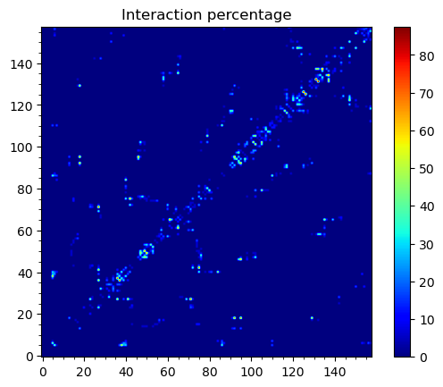
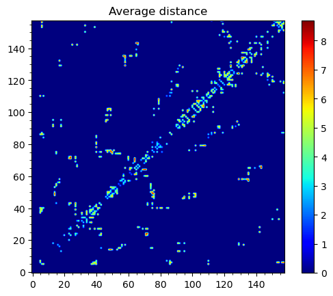
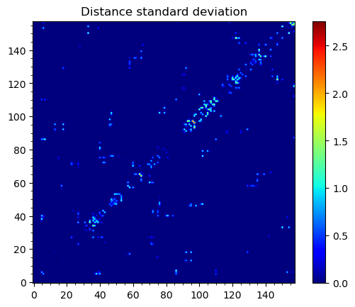
To obtain maps of interactions for the protein structure, we can use
showWaterBridgeMatrix(), which is equipped with three paramaters:
'percentage' (how often two residues were forming water bridges),
'distAvg' (how close there were on average), and 'distStd' (how
stable that water bridge was).
In [16]: showWaterBridgeMatrix(analysisAtomic, 'percentage')
In [17]: showWaterBridgeMatrix(analysisAtomic, 'distAvg')
In [18]: showWaterBridgeMatrix(analysisAtomic, 'distStd')
Raw data of the matrices can be obtained with calcWaterBridgeMatrix().
The type of the data in the matrix can be selected using the following
strings for the second argument: 'percentage', 'distAvg', 'distStd'.
In [19]: M1 = calcWaterBridgeMatrix(analysisAtomic, 'percentage')

In [20]: M2 = calcWaterBridgeMatrix(analysisAtomic, 'distAvg')

In [21]: M3 = calcWaterBridgeMatrix(analysisAtomic, 'distStd')
In [22]: M1
array([[ 0.  ,  0.  ,  0.  , ...,  0.  ,  0.  ,  0.  ],
       [ 0.  ,  0.  ,  0.  , ...,  0.  ,  0.  ,  0.  ],
       [ 0.  ,  0.  ,  0.  , ...,  0.  ,  0.  ,  0.  ],
       ...,
       [ 0.  ,  0.  ,  0.  , ...,  0.  , 12.5 , 31.25],
       [ 0.  ,  0.  ,  0.  , ..., 12.5 ,  0.  , 12.5 ],
       [ 0.  ,  0.  ,  0.  , ..., 31.25, 12.5 ,  0.  ]])
In [23]: M2
array([[0.        , 0.        , 0.        , ..., 0.        , 0.        ,
        0.        ],
       [0.        , 0.        , 0.        , ..., 0.        , 0.        ,
        0.        ],
       [0.        , 0.        , 0.        , ..., 0.        , 0.        ,
        0.        ],
       ...,
       [0.        , 0.        , 0.        , ..., 0.        , 4.58851337,
        5.82083416],
       [0.        , 0.        , 0.        , ..., 4.58851337, 0.        ,
        3.52366138],
       [0.        , 0.        , 0.        , ..., 5.82083416, 3.52366138,
        0.        ]])
In [24]: M3
array([[0.        , 0.        , 0.        , ..., 0.        , 0.        ,
        0.        ],
       [0.        , 0.        , 0.        , ..., 0.        , 0.        ,
        0.        ],
       [0.        , 0.        , 0.        , ..., 0.        , 0.        ,
        0.        ],
       ...,
       [0.        , 0.        , 0.        , ..., 0.        , 1.71697354,
        1.38650537],
       [0.        , 0.        , 0.        , ..., 1.71697354, 0.        ,
        1.27207112],
       [0.        , 0.        , 0.        , ..., 1.38650537, 1.27207112,
        0.        ]])
Statistical analysis for water bridges
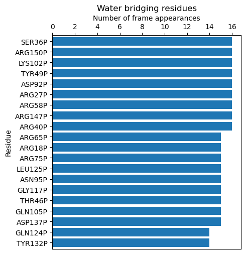
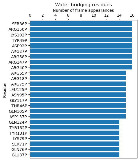
To visualize the results in a more accessible way, we can use the
calcBridgingResiduesHistogram() function, which will show how often each residue
was contributing to the water bridges in the trajectory.
In [25]: wb_res_hist = calcBridgingResiduesHistogram(waterBridges)

In [26]: wb_res_hist
[('LEU96P', 1),
 ('MET63P', 1),
 ('PHE152P', 1),
 ('LEU29P', 1),
 ('PRO130P', 1),
 ('PHE85P', 1),
 ('PRO54P', 1),
 ('ILE16P', 1),
 ('CYS148P', 1),
 ('VAL25P', 1),
 ('ILE77P', 1),
 .
 .
 ('ARG75P', 15),
 ('ARG18P', 15),
 ('ARG65P', 15),
 ('ARG40P', 16),
 ('ARG147P', 16),
 ('ARG58P', 16),
 ('ARG27P', 16),
 ('ASP92P', 16),
 ('TYR49P', 16),
 ('LYS102P', 16),
 ('ARG150P', 16),
 ('SER36P', 16)]
The clip option can be used to include different number of results on the histogram.
In [27]: calcBridgingResiduesHistogram(waterBridges, clip=25)
If we are interested in one particular residue, we can also use
calcWaterBridgesDistribution() to find their partners in water bridges.
Below we can see results for arginine 147 or aspartic acid 92 from chain P
using the nomenclature for them corresponding to the keys of the dictionary.
In [28]: calcWaterBridgesDistribution(waterBridges, 'ARG147P')
[('GLN122P', 8),
 ('ARG150P', 7),
 ('GLN143P', 6),
 ('LYS123P', 6),
 ('GLN124P', 5),
 ('ASP120P', 5),
 ('GLN144P', 3),
 ('THR140P', 2)]
In [29]: calcWaterBridgesDistribution(waterBridges, 'ASP92P')
[('ARG18P', 11),
 ('ASN95P', 10),
 ('SER94P', 5),
 ('MET91P', 5),
 ('ASP129P', 4),
 ('LEU13P', 3),
 ('CYS90P', 1)]
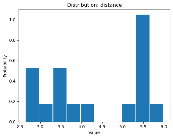
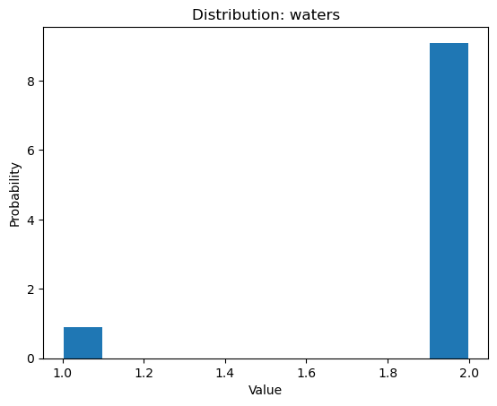
Once we select a pair of residues which are supported by interactions with water
molecules, we can use calcWaterBridgesDistribution() to obtain histograms
with results such as distances between them (metric='distance'), the number of
water molecules which were involved (metric='waters'), and information about
residue part which was involved in water bridges, i.e. backbone or side chain
(metric='location').
In [30]: calcWaterBridgesDistribution(waterBridges,  'ASP92P', 'ARG18P',
   ....:                              trajectory=trajectory, metric='distance')
   ....:
[5.3736005,
 5.3736005,
 5.167575,
 2.681302,
 5.371548,
 2.6318514,
 3.0394073,
 4.0884595,
 5.4406505,
 3.4112484,
 2.805657,
 5.4176636,
 3.5104342,
 5.991175,
 5.470093,
 3.4345005,
 3.6427624]
In [31]: calcWaterBridgesDistribution(waterBridges, 'ARG147P', 'GLN122P',
   ....:                                                      metric='waters')
   ....:
[2, 2, 2, 2, 2, 2, 2, 2, 1, 2, 2]
In [32]: calcWaterBridgesDistribution(waterBridges, 'ARG147P', 'GLN122P',
   ....:                              trajectory=trajectory, metric='location')
   ....:
{'ARG147P': {'backbone': 7, 'side': 86},
'GLN122P': {'backbone': 21, 'side': 25}}
Save results as PDB file
The results can be stored as a PDB file using savePDBWaterBridges()
(single PDB file, single frame) or using savePDBWaterBridgesTrajectory()
to save all the results (large number of frames saved each independently).
5kqm_all_sci_multi_0.pdb 5kqm_all_sci_multi_1.pdb .. 5kqm_all_sci_multi_15.pdb
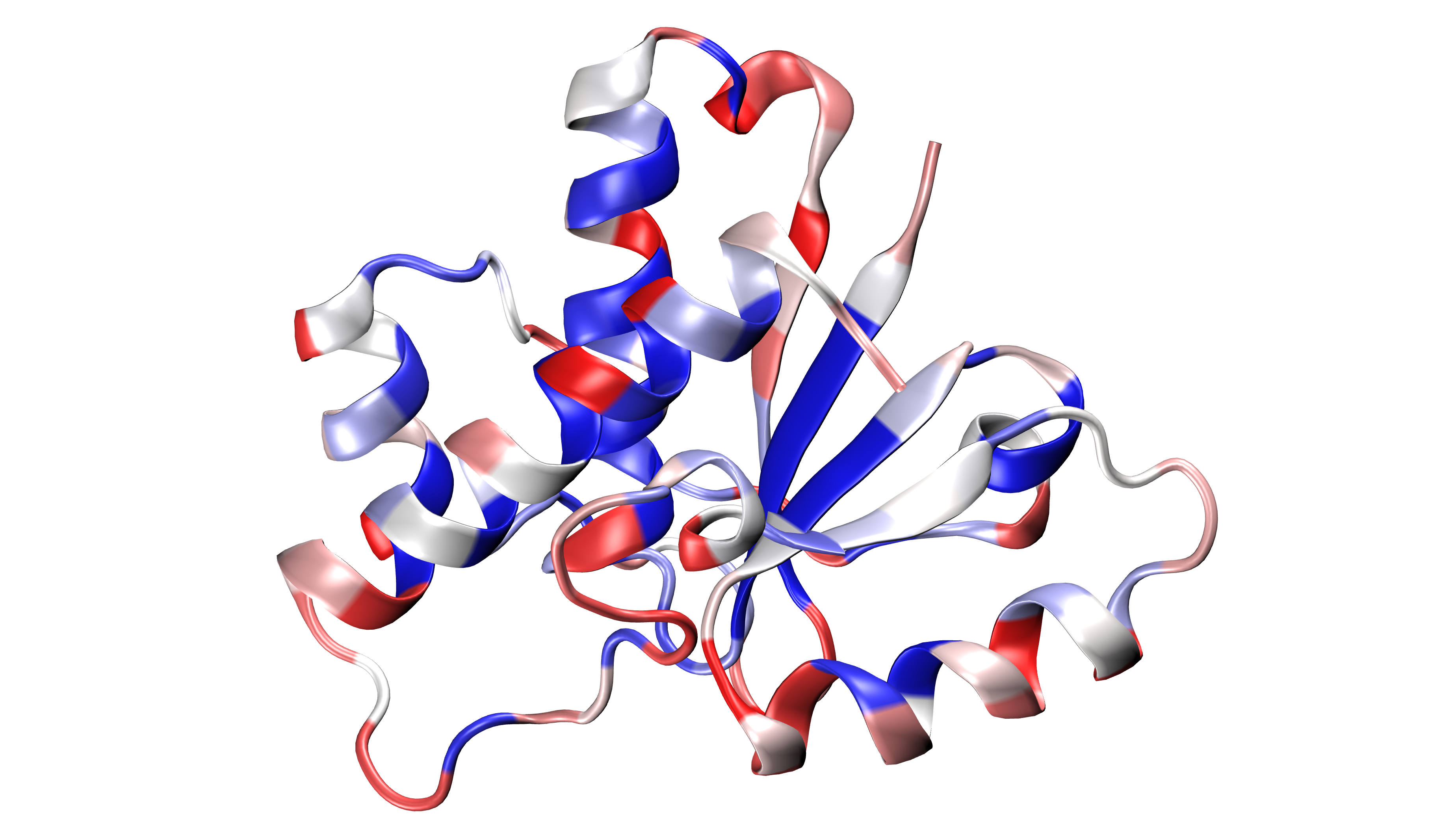
Those results can be displayed in any program for visualization. The results
for the protein structure will be storage in the B-factor (*beta*) column (average values of
contributions of each residue in water bridging) and Occupancy column
(results for particular frame). Water molecules will be included in each frame.
In [33]: savePDBWaterBridges(waterBridges[0], coords_traj, PDBtraj_file[:-4]+'_frame0.pdb')

In [34]: savePDBWaterBridgesTrajectory(waterBridges, coords_traj,
   ....:                               filename=PDBtraj_file[:-4]+'_multi.pdb',
   ....:                               trajectory=trajectory)
   ....:
Results saved in PDB file can be displayed as follows:

