Gaussian Network Model (GNM)

This example shows how to perform GNM calculations using an X-ray structure of ubiquitin. A GNM instance that stores the Kirchhoff matrix and normal mode data describing the intrinsic dynamics of the protein structure will be obtained. GNM instances and individual normal modes (Mode) can be used as input to functions in prody.dynamics module.

See [Bahar97] and [Haliloglu97] for more information on the theory of GNM.

[Bahar97]

Bahar I, Atilgan AR, Erman B. Direct evaluation of thermal fluctuations in protein using a single parameter harmonic potential. Folding & Design 1997 2:173-181.

[Haliloglu97]

Haliloglu T, Bahar I, Erman B. Gaussian dynamics of folded proteins. Phys. Rev. Lett. 1997 79:3090-3093.

Parse structure

We start by importing everything from the ProDy package:

In [1]: from prody import *

In [2]: from matplotlib.pylab import *

In [3]: ion() # turn interactive mode on

First we parse a PDB file by passing its identifier to parsePDB() function. Note that if file is not found in the current working directory, it will be downloaded.

In [4]: ubi = parsePDB('1aar')

In [5]: ubi
Out[5]: <AtomGroup: 1aar (1218 atoms)>

This file contains 2 chains, and a flexible C-terminal (residues 71-76). We only want to use Cα atoms of first 70 residues from chain A, so we select them:

In [6]: calphas = ubi.select('calpha and chain A and resnum < 71')

In [7]: calphas
Out[7]: <Selection: 'calpha and chai...and resnum < 71' from 1aar (70 atoms)>

See definition of “calpha”, “chain”, and other selection keywords in Atom Selections.

Note that, flexible design of classes allows users to select atoms other than alpha carbons to be used in GNM calculations.

Build Kirchhoff matrix

Instantiate a GNM instance:

In [8]: gnm = GNM('Ubiquitin')

We can build Kirchhoff matrix using selected atoms and GNM.buildKirchhoff() method:

In [9]: gnm.buildKirchhoff(calphas)

We can get a copy of the Kirchhoff matrix using GNM.getKirchhoff() method:

In [10]: gnm.getKirchhoff()
Out[10]: 
array([[11., -1., -1., ...,  0.,  0.,  0.],
       [-1., 15., -1., ...,  0.,  0.,  0.],
       [-1., -1., 20., ...,  0.,  0.,  0.],
       ...,
       [ 0.,  0.,  0., ..., 20., -1., -1.],
       [ 0.,  0.,  0., ..., -1., 21., -1.],
       [ 0.,  0.,  0., ..., -1., -1., 12.]])

Parameters

We didn’t pass any parameters, but GNM.buildKirchhoff() method accepts two of them, which by default are cutoff=10.0 and gamma=1.0, i.e. buildKirchhoff(calphas, cutoff=10., gamma=1.)

In [11]: gnm.getCutoff()
Out[11]: 10.0

In [12]: gnm.getGamma()
Out[12]: 1.0

Note that it is also possible to use an externally calculated Kirchhoff matrix. Just pass it to the GNM instance using GNM.setKirchhoff() method.

Calculate normal modes

We now calculate normal modes from the Kirchhoff matrix.

In [13]: gnm.calcModes()

Note that by default 20 non-zero (or non-trivial) modes and 1 trivial mode are calculated. Trivial modes are not retained. To calculate different numbers of non-zero modes or to keep zero modes, try gnm.calcModes(50, zeros=True).

Normal mode data

Get eigenvalues and eigenvectors:

In [14]: gnm.getEigvals().round(3)
Out[14]: 
array([ 2.502,  2.812,  4.366,  5.05 ,  7.184,  7.65 ,  7.877,  9.08 ,
        9.713, 10.132, 10.502, 10.644, 10.888, 11.157, 11.285, 11.632,
       11.78 , 11.936, 12.006, 12.218])

In [15]: gnm.getEigvecs().round(3)
Out[15]: 
array([[-0.064, -0.131, -0.245, ..., -0.256,  0.538, -0.   ],
       [-0.073, -0.085, -0.19 , ...,  0.006, -0.069,  0.032],
       [-0.076, -0.043, -0.135, ...,  0.017, -0.047,  0.018],
       ...,
       [-0.092,  0.064,  0.105, ...,  0.032, -0.042,  0.006],
       [-0.07 ,  0.099,  0.054, ...,  0.031,  0.024, -0.014],
       [-0.081,  0.135,  0.124, ...,  0.013, -0.04 , -0.018]])

Get covariance matrix:

In [16]: gnm.getCovariance().round(2)
Out[16]: 
array([[ 0.08,  0.02,  0.01, ..., -0.01, -0.01, -0.01],
       [ 0.02,  0.02,  0.01, ..., -0.  , -0.  , -0.01],
       [ 0.01,  0.01,  0.01, ...,  0.  , -0.  , -0.  ],
       ...,
       [-0.01, -0.  ,  0.  , ...,  0.01,  0.01,  0.01],
       [-0.01, -0.  , -0.  , ...,  0.01,  0.01,  0.02],
       [-0.01, -0.01, -0.  , ...,  0.01,  0.02,  0.05]])

Note that covariance matrices are calculated using the available modes in the model, which is the slowest 20 modes in this case. If the user calculates M modes, these M modes will be used in calculating the covariance matrix.

Individual modes

Normal mode indices start from 0, so slowest mode has index 0.

In [17]: slowest_mode = gnm[0]

In [18]: slowest_mode.getEigval().round(3)
Out[18]: 2.502

In [19]: slowest_mode.getEigvec().round(3)
Out[19]: 
array([-0.064, -0.073, -0.076, -0.112, -0.092, -0.143, -0.164, -0.205,
       -0.24 , -0.313, -0.192, -0.152, -0.066, -0.07 , -0.025, -0.031,
        0.001, -0.006, -0.015,  0.027,  0.042,  0.055,  0.063,  0.09 ,
        0.09 ,  0.069,  0.132,  0.175,  0.145,  0.121,  0.195,  0.218,
        0.158,  0.217,  0.245,  0.214,  0.225,  0.171,  0.2  ,  0.151,
        0.102,  0.043, -0.029, -0.064, -0.072, -0.086, -0.09 , -0.078,
       -0.057, -0.011,  0.016,  0.061,  0.058,  0.043,  0.029,  0.013,
        0.004,  0.011, -0.013, -0.037, -0.05 , -0.059, -0.07 , -0.094,
       -0.094, -0.099, -0.097, -0.092, -0.07 , -0.081])

By default, modes with 0 eigenvalue are excluded. If they were retained, slowest non-trivial mode would have index 6.

Access hinge sites

Hinge sites identified from all calculated modes (n_modes defined when calling gnm.calcModes()) can be obtain by using the following command.

In [20]: hinges = calcHinges(gnm)

In [21]: hinges[:5]
Out[21]: [0, 1, 2, 3, 4]

Hinge sites in the slowest mode can be obtained by:

In [22]: calcHinges(gnm[0])
Out[22]: [16, 18, 42, 49, 57]

Hinge sites identified from multiple modes (e.g. 2 modes) can be accessed by:

In [23]: calcHinges(gnm[:2])
Out[23]: [3, 14, 16, 18, 25, 42, 43, 46, 47, 48, 49, 57, 65]

These numbers correspond to node indices in the GNM object, which does not know anything about the original atoms. In order to get the residue numbers corresponding to these hinges, we can index the resum array with the hinges list as follows:

In [24]: resnums = calphas.getResnums()

In [25]: mode2_hinges = calcHinges(gnm[1])

In [26]: resnums[mode2_hinges]
Out[26]: array([ 4, 15, 26, 44, 47, 48, 49, 66])

Plot results

ProDy plotting functions are prefixed with show. Let’s use some of them to plot data:

Contact Map

In [27]: showContactMap(gnm);

Cross-correlations

In [28]: showCrossCorr(gnm);

Slow mode shape

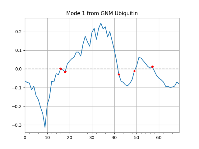
By default, hinge sites will be shown in mode shape plot indicated by red stars, and it can be turned off by setting hinges=False. The option zero=True is to turn on the reference line of zero.

In [29]: showMode(gnm[0], hinges=True, zero=True);

In [30]: grid();

Square fluctuations

In [31]: showSqFlucts(gnm[0], hinges=True);

Protein structure bipartition

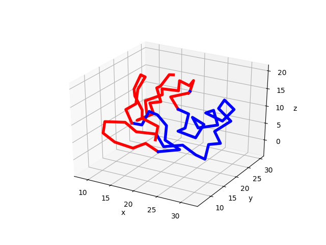
Given a GNM mode, protein structure can be partitioned into two parts that move with respect to each other. The function showProtein() can take a GNM mode as input and visualize the bipartition.

In [32]: showProtein(calphas, mode=gnm[0]);